¶ LuSim Product Overview
¶ What LuSim is
LuSim is a web-based 3D solar simulation platform built by LuciSun. You open it in a browser, build a 3D scene (terrain, buildings, trees, PV modules), and the GPU computes how sunlight reaches every cell of every module and every point of every object over a full year.
The core promise: replace a hand-built mix of CAD geometry, PVsyst sims, BIPV mock-ups and Python scripts with one integrated tool that goes from scene to validated heatmap-and-graph deliverables.
LuSim simulates direct, diffuse and reflected irradiance on arbitrary 3D scenes, with cell-level granularity on PV modules.
¶ What LuSim is not
To set expectations clearly for the beta:
- Not an energy yield simulator. LuSim outputs irradiance and irradiation (W/m² and Wh/m²). DC/AC power, electrical model, mismatch losses, inverter behavior, degradation — none of that yet. PVsyst still owns the energy side.
- Not a CAD tool. You instance meshes, you don’t draw them. Complex geometry comes in as
.objfiles prepared elsewhere. - Not a financial / LCOE tool. No costs, no tariffs, no payback.
- Not a weather model. It reads weather; it doesn’t generate it.
- Not a meshing tool. UV maps and clean topology must be ready before import.
¶ Where LuSim is heading
LuSim is the geometry-and-irradiance core of a wider LuciSun stack. Things on the roadmap (some partially in code, some planned):
- Energy chain — module-level DC, string mismatch, inverter, system losses on top of the irradiance backbone.
- Semi-transparent BIPV — modules that transmit light to the ground plane (agrivoltaics, glazing).
- Custom BRDF / BTDF materials for accurate reflective and translucent surfaces.
- PVGIS connector for one-click weather data.
- Report generator — automated export of heatmaps, graphs and numerical tables.
- Faster, larger variants sweeps without browser memory limits.
If a feature isn’t in this guide, assume it isn’t in this build yet.
¶ Core Platform Philosophy
Four ideas drive design decisions:
-
Geometry-first. Everything in LuSim revolves around a 3D scene. Shading and reflections come from real geometry, not from analytical row-to-row formulas. Anything you can put in a
.objyou can shade with. -
GPU as the simulation engine. Shading and view-factor sampling run as WebGL shaders. That’s how a year-long simulation on hundreds of cells fits in seconds-to-minutes inside a browser tab — but it’s also why a discrete GPU and hardware acceleration in the browser matter.
-
Reusable building blocks. Locations, meshes, PV modules and materials live in a database and are pulled into cases by reference. You build a library once, then assemble cases from it.
-
Baseline + variants. Trade-off studies (tilt, GCR, albedo, position…) are first-class. You define a baseline and only the deltas per variant — instead of N copies of a full scene.
¶ Integration with LuData (planned, not exposed yet)
LuSim will pull its environmental inputs from LuData, LuciSun’s data layer:
- Irradiance time series — hourly BNI / DNI_circ / DHI_iso (Hay-decomposed) per location, replacing the current manual
.irrupload. - Terrain — site-specific elevation grids feeding the default
Terrain_0/Terrain_1objects. - Horizon profile — far-field horizon mask per location (PVGIS-style horizon files).
These hooks exist in the data model today but are not wired to the UI. Until then, expect to feed weather manually (.irr file) and to live with the default flat terrains.
¶ Platform Architecture
| Layer | Stack | Role |
|---|---|---|
| Frontend | Three.js, custom WebGL shaders, Bootstrap, Plotly | 3D viewport, shading and view-factor shaders, heatmap and graph rendering |
| Backend | Python 3, Flask, Gunicorn + Gevent | Auth, scene lifecycle, solar geometry (via pvlib), mesh processing, file I/O |
| Database | MySQL | User accounts, locations, modules, materials, case metadata |
| Storage | S3-compatible | Meshes, textures, .irr weather files, case configs, simulation results |
| Heavy math | pvlib, pandas, numpy, scipy, pymeshlab | Sun position, Hay decomposition, mesh prep |
The split is deliberate: solar physics on the Python side (validated libraries, deterministic outputs), everything geometric and pixel-counting on the GPU side.
¶ Usage Model
A typical session looks like this:
- Set up your library (one-time, then reused).
- Add a location (
.irrweather file). - Import the meshes you’ll need (OBJ).
- Make sure the PV modules you need are in the shared module DB.
- Add any custom materials.
- Add a location (
- Create a case — pick a location, give it a name, start from an empty scene or a YAML template.
- Build the scene — instance meshes, place PV layouts and POAs, assign materials.
- Define targets — what surfaces should LuSim compute irradiance on, and at what mesh resolution.
- Define variants (optional) — deltas from baseline for trade-off studies.
- Run — Play, watch the progress bar.
- Inspect — heatmaps for visual sanity, analytics for numbers and graphs.
- Export — download CSVs and figures, or export the case as a zip for archive/sharing.
Cases live server-side. You can close the browser and reopen them later from any machine.
¶ Who LuSim is For
LuSim is designed around three personas:
| Persona | Why they’d use LuSim |
|---|---|
| PV / BIPV designer | Quantify shading from buildings, vegetation, neighbouring structures on a real 3D scene. Compare orientations, tilts, GCR or row-spacing variants on the same baseline. |
| R&D / solar physicist | Test specific irradiance components (isolate BTI, DTI_circ, reflected, etc.) on controlled scenes. Validate models against measurements with cell-level granularity. |
| Agrivoltaics / niche application engineer | Evaluate ground-level irradiance under tracker arrays, in greenhouses, or behind reflective surfaces — cases that classical PV simulators don’t handle natively. |
In all three cases the user is comfortable with solar terminology (DNI, DHI, GHI, POA, GCR…) and at ease editing a YAML file when needed.
LuSim is not aimed at end-clients producing financial reports, at homeowners sizing rooftop systems, or at GIS workflows over large geographic areas.
¶ How This Documentation Is Structured
The wiki is organised into five pages. Read them in order on your first visit; refer back as needed afterwards.
- Platform Overview (this page) — what LuSim is, the architecture, who it’s for.
- Core Concepts — the physics LuSim relies on, with the key formulas:
- Sun position (NREL SPA via pvlib
solarposition.get_solarposition). - Hay/Davies diffuse decomposition — splits DHI into a circumsolar component aligned with the sun and an isotropic component from the sky dome:
DHI = DNI_circ + DHI_iso, with the Hay anisotropy indexA_i = BNI / I0controlling the split (I0= extra-terrestrial normal irradiance).
- POA transposition (via
pvlib.irradiance.get_total_irradiance/haydavies):BTI = BNI · cos(θ_i)whereθ_iis the angle of incidence on the panel.DTI_circ = DHI · A_i · cos(θ_i) / cos(θ_z)(circumsolar treated as direct).DTI_iso = DHI · (1 − A_i) · (1 + cos(β)) / 2(isotropic, β = tilt).POA_ground = GHI · ρ · (1 − cos(β)) / 2for the simple ground-reflected term (ρ = albedo).
- Total POA =
BTI + DTI_circ + DTI_iso + POA_ground, modulated by per-cell shading factors and per-vertex view factors computed on the GPU. - View factors — sky-dome and ground sampled with hemispherical GPU renders (180° fish-eye); each vertex carries
sky_view_factor,DHI_view_factorandDNI_view_factor, transferred to PV cells via mesh interpolation. - Geometric vs effective shading —
geometriccounts the shaded area;effectiveapplies the module’s electrical response (relevant once string-power outputs ship).
- Sun position (NREL SPA via pvlib
- User Manual — step-by-step walkthrough of the interface using the three example projects (shading, bifacial, agrivoltaics). This is the page you keep open while you use LuSim.
- FAQ — short answers to common pitfalls: hardware acceleration, OBJ import errors, variant memory limits, weather file format, missing modules in the DB, etc.
- Support & Issue Reporting — where to log bugs (the shared spreadsheet first, Gitlab tickets for prioritised ones), what info to include (case name, variant, browser, GPU), and how to reach the LuSim team.
One convention to memorize before going further: LuSim uses a right-handed axis system with +X = South, +Y = East, +Z = Up, and a POA orientation of 0° = facing south, −90° = facing east. The full convention table lives on the User Manual page.
¶ LuSim — User Manual (v0.22)
Welcome to the LuSim beta! LuSim is a web-based 3D solar simulation tool. You build a scene in your browser, place PV modules, hit Play, and the GPU computes how sunlight (direct, diffuse and reflected) reaches every cell of your modules and every point of your scene. This can of course be adjusted depending on the level of detail and complexity, which will affect the accuracy as well as the computational load of the tool. You can then visualise results as heatmaps or download them as time-series data.
This guide walks you through everything you need as a beta tester. We use three example projects to cover the main use-cases:
- Shading analysis — e.g. a BIPV roof with nearby buildings and trees.
- Bifacial gain — flat ground arrays with reflective patches.
- Agrivoltaics — trackers above an orchard.
The flow is always the same four steps:
- Build the 3D scene (terrain + objects + PV).
- Define what you want to measure (targets) and any what-if cases (variants).
- Run the simulation.
- Inspect the results.
Heads-up: this is a beta build. Expect rough edges. Please log anything you find in the shared bug-tracking spreadsheet so we can sort, prioritise, and turn them into tickets.
¶ Conventions
Read this once. It saves you a lot of confusion later.
¶ Coordinate system
LuSim uses a right-handed coordinate system with the following compass mapping (always visible as the small RGB axis gizmo in the 3D view):
| Axis | Color | Direction | Positive direction | Negative direction |
|---|---|---|---|---|
| X | Red | North–South | South (+X) | North (−X) |
| Y | Green | East–West | East (+Y) | West (−Y) |
| Z | Blue | Vertical | Up (+Z) | Down (−Z) |
Practical consequences:
- A position of
(10, 0, 0)is 10 m south of the origin. - A position of
(0, 10, 0)is 10 m east of the origin. - A
Rectangular patternwithdX = 5, nX = 5is spaced 5 m apart along the N–S line, anddY = 4, nY = 9is 4 m apart along the E–W line. - A POA with Orientation = 0° faces South (so the panel normal points south).
- A POA with Orientation = −90° faces East.
- Orientation grows positive going South → West → North and negative going South → East → North.
- Tilts are around the local horizontal axis of the POA; +Z is the panel’s “up”.
- Rotations are applied in the ZYX order (yaw → pitch → roll).
¶ Irradiance components
LuSim distinguishes three families of light and three sources of each.
Three components (Hay decomposition):
| Symbol | Name | Meaning |
|---|---|---|
| BNI | Beam Normal Irradiance | Direct sunbeam from the sun’s direction, measured on a plane perpendicular to the sun (W/m²). Other tools often call this DNI. |
| DNI_circ | Circumsolar diffuse | Diffuse light arriving from a halo around the sun (treated as coming from the sun direction by Hay). |
| DHI_iso | Isotropic diffuse | Diffuse light arriving uniformly from the sky dome. |
These three values are read from your location’s .irr weather file at each time step. Together with GHI (Global Horizontal) and DHI (total Diffuse Horizontal), they define the sky for that moment.
Three sources of arriving light, for any target surface:
| Source | What it represents |
|---|---|
| Sun | Direct sunbeam + circumsolar arriving from the sun’s direction. Shading applies. |
| Sky | Isotropic diffuse from the visible sky dome (depends on how much sky the target “sees”). |
| Albedo | Light bouncing off the ground/objects toward the target. |
Component on the tilted target plane (POA):
When the three components are projected onto your actual tilted PV surface or object face, you get their transposed counterparts:
| Symbol | Meaning |
|---|---|
| BTI | Beam Transposed Irradiance — BNI as seen by the tilted surface |
| DTI_circ | Circumsolar diffuse on the tilted surface |
| DTI_iso | Isotropic diffuse on the tilted surface |
Each is reported with three flavors:
*_unshaded— what would arrive with no obstacles.*_shaded— what actually arrives after shading by the scene.*_reflected— albedo-reflected contribution.
Naming quirk in the UI: the heatmap and analytics panels label the breakdown rows BTI / DTI_circ / DTI_iso (the on-plane values you actually see), while the override fields are labeled BNI / DNI circ / DHI iso (the source values from the weather file). They describe the same components at two different stages.
¶ Units
- Distances: meters (m).
- Angles: degrees (°).
- Irradiance: W/m².
- Irradiation (energy): Wh/m².
- Time: depending on the panel, UTC or local time — both are toggleable on the step-vector window (F1).
¶ 1. Getting Started
¶ 1.1 Logging in
LuSim is now invitation-only: an admin invites you by email, you click the link, and you set your own password. There are no shared accounts anymore.
If you can’t log in, ping an admin to resend an invite. From the main interface, the Admin button (top right) is visible only if you have admin privileges.
¶ 1.2 The interface

The top bar has three groups of buttons:
| Group | Buttons | Purpose |
|---|---|---|
| Left | New, Open, Save | Create, open, save your case |
| Center | Database, Options, Play | Manage shared/personal libraries, edit your scene, run the simulation |
| Right | Heatmap, Analytics, Admin, Logout | Post-process and account |


The big area below is your 3D view. All panels open as semi-transparent overlays so you keep seeing your scene.
¶ 1.3 Function keys
Toggle floating windows and helpers with the F-keys:
| Key | Window |
|---|---|
| F1 | Step-vector window (yield / direct shading / diffuse / DNI view factor) |
| F2 | Variants dashboard |
| F3 | GPU texture viewer (debug for spherical-view computations) |
| F4 | Auxiliary 3D canvas (object/layout previews — usually opens automatically) |
| F5 | Picked-point info window (use after a double-click in the 3D view) |
| F7 / F8 | Show / hide auxiliary GPU meshes |
| F9 | Recompute the terrain height heatmap (debug) |
| F10 | Export the current rectangular POA as Adapted_topography.yaml |
| F11 | Dump a sample heatmap PNG (debug) |
F6 is wired up in the UI but currently inactive in this build. Ignore it.
¶ 2. Build the 3D Scene
¶ 2.1 Create a new case
Click New  . The dialog has three fields:
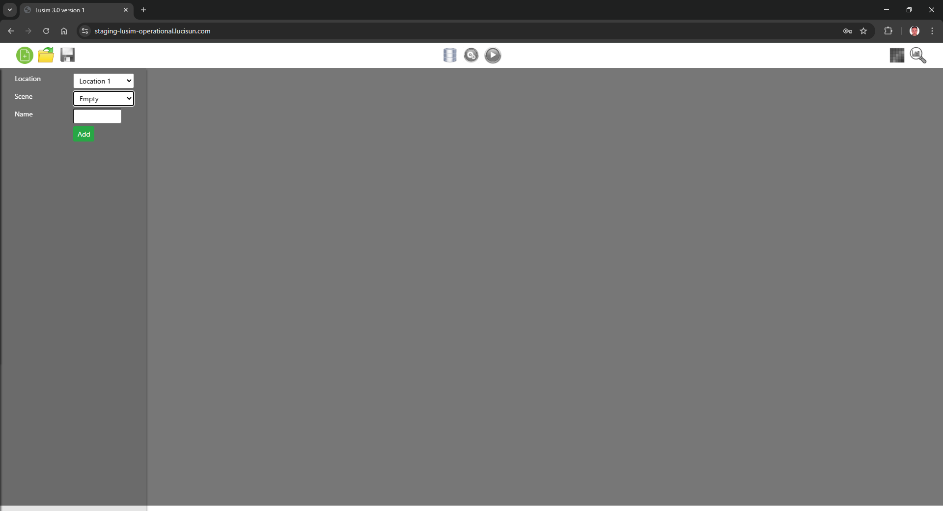
- Location — pick from your locations (see Annex I).
- Scene —
Empty(build interactively) orFrom file(YAML template, for advanced users — see Annex V). - Name — unique. Examples in this guide:
Manual – Shading,Manual – Bifacial,Manual – Agrivoltaics.
An empty scene comes with two default terrains:
- Terrain_0 — outer ground, up to 2 km × 2 km.
- Terrain_1 — inner ground, 100 m × 100 m.
No material is applied yet.
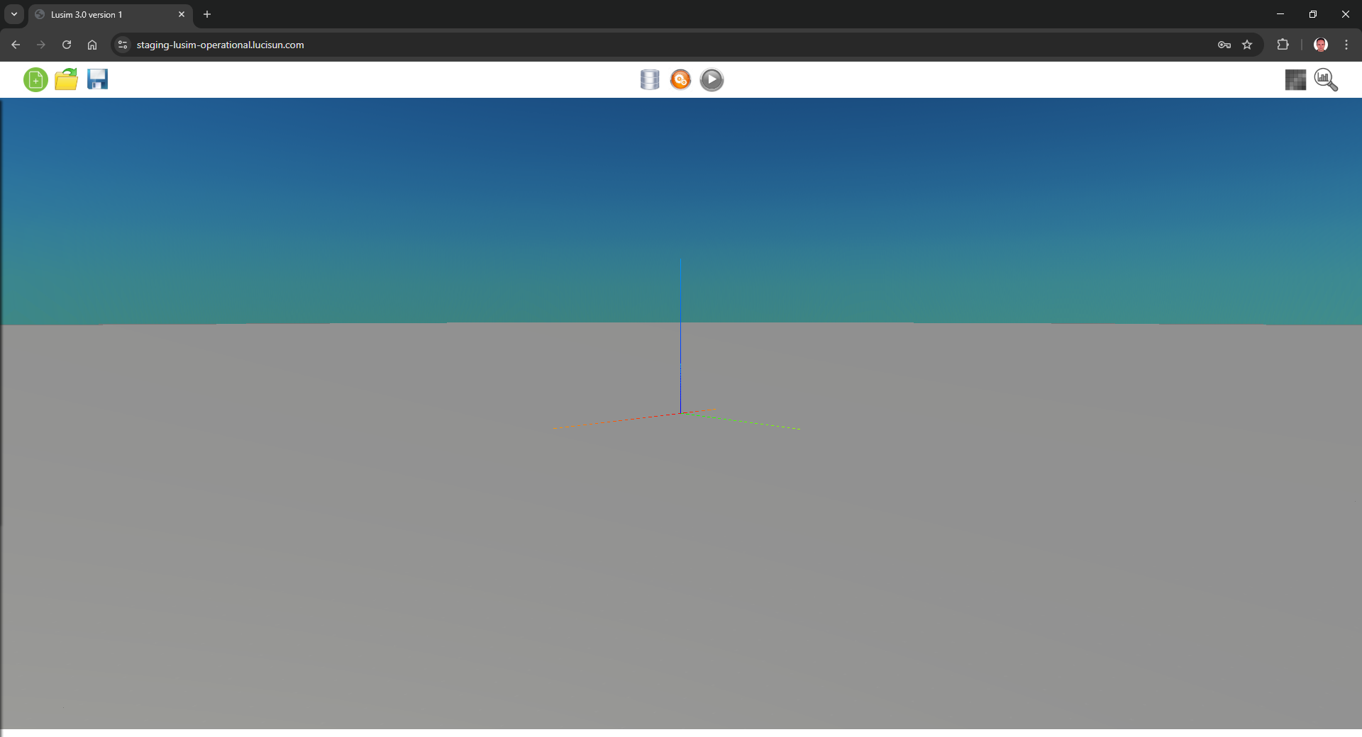
Two more buttons appear:
- Save
 — saves or exports the case.
 - Options
 — opens the editing panel.
¶ 2.2 The Options panel
Three sections:

- Scene — add/modify/delete objects and PV generators.
- Kinematics — time resolution, tracker laws.
- Simulation — targets and variants (see §6).
¶ 2.3 Apply a material to the default terrains
Options → Scene → Objects → Select terrain_0 → Material = Ground → Modify. Repeat for terrain_1.


Always click Modify and wait for the “changes applied” confirmation before switching to another object. Anything you change before clicking Modify is preview-only.
¶ 3. Example 1 — Shading Analysis (BIPV)
We’ll add a house, two buildings, two trees, then put PV on the roof.
¶ 3.1 Mesh vs Object
- A mesh lives in your DB (a 3D model file).
- An object is an instance of a mesh placed in the scene.
The same mesh can be instanced many times with different positions, scales and rotations.
¶ 3.2 Object fields
Options → Scene → 3D objects:

| Field | What it does |
|---|---|
| Select | New Object or an existing one |
| Mesh | Mesh from your DB (Annex III to add new ones) |
| Material | Apply at creation (optional) |
| Kinematics | Fixed (1-axis tracker is reserved for PV generators in the UI) |
| Type | Single object, Rectangular pattern, or User pattern |
| Position | (x, y, z) in meters — remember +X south, +Y east |
| Rotation | Degrees (x, y, z), applied in ZYX order |
| Scale | Per-axis multiplier |
| Name | Must be unique |
| Normalize? | Reserved for certain terrains |
| Receptor? | Virtual object — doesn’t cast shadow but receives irradiance (e.g. a tree’s convex hull) |
Rectangular pattern adds:
| Field | What it does |
|---|---|
| dX | Spacing in X (N–S), m |
| dY | Spacing in Y (E–W), m |
| nX | Count in X (fixed after creation) |
| nY | Count in Y (fixed after creation) |
| theta | Z-rotation of the whole pattern (deg, positive clockwise when viewed from above) |
User pattern adds:
| Field | What it does |
|---|---|
| Number | How many instances — start sharing one position/rotation/scale, then edit each by Id |
¶ 3.3 Place the three objects
- House —
Single objectat(0, 0, 0), no rotation, scale(1, 1, 1), nameHouse.

- Buildings —
Rectangular pattern,nY = 2, nX = 1,dY = 30 m, rotation(0, 0, −90°).

- Trees —
User pattern,Number = 2, initial scale(3, 3, 3), initial position(20, 0, 0). Both overlap until you edit them individually.

¶ 3.4 Edit instances individually
Re-select the object, then choose its Id (0-based). All fields refresh to the stored values for that instance.

For our trees:
| Id | Position | Scale |
|---|---|---|
| 0 | (12, −7, 0) | (3, 3, 3) |
| 1 | (12, 6, 0) | (4, 4, 4) |
Click Modify for each Id before switching to the next.

¶ 3.5 PV generator: Layout then POA
A PV generator is built in two steps:
- Layout — the matrix of modules (and their wiring). Reusable across cases.
- POA (Plane of Array) — where that layout sits in the scene.
¶ Create a Layout
Options → Scene → PV generators → Layouts:

| Field | What it does |
|---|---|
| PV module | Choose from DB (shared with all users) — Annex II to add new ones |
| Option | Rectangular (the only one in the UI; advanced via YAML) |
| Orientation | Portrait or Landscape |
| dX, dY | Module spacing in local X (right when viewed from above) and Y (m) |
| nX, nY | Module count |
| z | Plane height above the local axis (typically 0; useful for trackers) |
| Name | Unique |
The auxiliary preview is rotatable (left-click drag inside) and pannable (right-click drag on its frame).

Local axis tip: Layout X points to the right when you look at the module from above (i.e. from +Z). This matters when you later rotate the POA — your tilt will be around that X.
¶ Decide where to mount it
Press F5, then double-click in the middle of the roof. The info window shows the picked point and its normal:

¶ Create the POA
Options → Scene → PV generators → Plane of arrays → New POA:
| Field | What it does |
|---|---|
| Layout | Pick the layout you just made |
| Structure | Optional mounting structure: Predefined (e.g. Vertical PV — 3 parameters) or Customized |
| Kinematics | Fixed or 1-axis tracker (tracker needs a defined rotation axis) |
| Type | Single POA / Rectangular pattern / User pattern |
| Option | Basic, Pointer, or Detailed — see below |
| Name | Unique |
Three placement options:
- Basic — simplest. Set Orientation (0° = south, −90° = east), Tilt (°), and GND dist (m, lowest point of the array to the ground).
- Pointer — best for BIPV. Double-click any surface; the orientation snaps to that surface’s normal. Use Gap to set the offset (m).
- Detailed — full manual control: Position
(x, y, z)and Rotation(x, y, z)in ZYX order.
For the BIPV example, use Pointer, click the roof, name it P1.


¶ 4. Example 2 — Bifacial Gain with Different Albedos
This example builds reflective patches on the ground in front of bifacial modules and sweeps several parameters. We use YAML templates here, both for the scene and for the variants, because creating dozens of individually-positioned patches by hand is painful.
¶ 4.1 Trade-off matrix
Baseline values in bold.
| Parameter | Values |
|---|---|
| Ground distance (m) | 0.2, 0.5, 1, 1.5 |
| Tilt (°) | 0, 10, 20, 30, 45, 60, 75, 90 |
| Orientation (°) | 0, 180, −90, 90, −45, 45 |
| Albedo | 0.5, 0.8 |
| Ground Coverage Ratio (GCR) | 0.5, 0.6, 0.7 |
| Ground Reflective Ratio (GRR) | 0, 0.25, 0.5, 0.75, 1.0 |
| Reflective surface position | A, B, C, D |
Memory note: running ~50+ variants at once tends to crash the browser. Vary one parameter at a time.
¶ 4.2 Patch geometry (baseline)
Module DMEGC_DM545M10-B72HSW(1500V), 2V portrait → string length 4.57 m. We reuse a Patch_4x30.obj mesh (4 m × 30 m) for both reflective and non-reflective stripes.

Numbers:
- GCR 50 % → row spacing = 9.14 m.
- GRR 25 % → reflective stripe = 2.285 m wide, non-reflective stripe = 6.855 m.
- Scale the 4 m base patch by
0.57125for the reflective and1.71375for the non-reflective. - Y spacing = 30 m between rows.
¶ 4.3 Load the scene from YAML
Click New → From file → pick the YAML. The template defines:
- Objects S1 and S2 (both using
Patch_4x30.obj— must already be in your DB). - Layout L1: 26 × 2 modules of the DMEGC, 2 cm spacing, 2V portrait, two series strings of 26 modules each (upper and lower row).

¶ 4.4 Tidy the default terrain
Delete terrain_1 (Options → Scene → Objects → select → Delete):


Assign materials:
| Object | Material |
|---|---|
| terrain_0 | Ground |
| S1 (reflective) | White stones |
| S2 (non-reflective) | Ground |


Save before going on.
¶ 4.5 Close the gap by scaling Terrain_0
Patches span 70.835 m (X, N–S) × 90 m (Y, E–W) but the hole is 100 × 100. Scale terrain_0 by (0.70835, 0.9, 1) and click Modify:

¶ 5. Example 3 — Agrivoltaics Irradiance
This one uses YAML because trackers aren’t in the UI yet.
Watch out: the YAML loader does not check whether the meshes/modules you reference exist in your DB. Verify by hand first.
¶ 5.1 Scene definition

- Trees: rectangular pattern of
Tree_T.obj,5 × 9,dX = 5 m(N–S),dY = 4 m(E–W). - PV: layout
Brand_Model, 20 modules in 1V, rectangular pattern of 9 POAs.

Two things new here:
kinematics: 1_axis_trackerplus an explicit rotation axis (no backtracking, rotation limits applied).diffuse_shadingstep vector usesitem_kinematicswith 10 rotation steps so the diffuse computation accounts for the tracker’s motion.

Result:

Set both terrains to Ground. Press F1 and slide through time steps — the trackers animate:

¶ 6. Targets and Variants
A target is where irradiance is computed. LuSim runs two engines:
- Direct shading — parallel rays, cell-level granularity on PV modules.
- Diffuse + albedo — 180° hemispherical view sampled on mesh vertices, transferred to cells afterwards.
¶ 6.1 Shading example — PV target
Options → Simulation → GPU toolset → Strings. Pick strings in the menu, or Ctrl + click directly on modules in the 3D view to add/remove them.

You’ll see two target categories: Direct shading and Diffuse and albedo. Pick the front side of the modules for both, with Medium mesh resolution for the diffuse one.
Mesh resolution = average triangle size on the surface:
| Preset | Size |
|---|---|
| Low | 1.0 m |
| Medium | 0.5 m |
| High | 0.25 m |
| Custom | your value |

¶ 6.2 Shading example — Object target
Options → Simulation → GPU toolset → Objects → House_0 → irradiance with detail Source (use the original mesh as the evaluation grid).

Click Create Set. The Play button lights up.

¶ 6.3 Variants
A variant is a delta from the baseline scene: hide/show, move, scale, rotate, switch material… You can also vary kinematics, targets and master/slave relationships, but those are less battle-tested.
Options → Simulation → Variants → name it v1 → Add:

Click Modify (or F2) to open the dashboard:

Pick variant v1, then trees_0. The element is highlighted in white. Click the visibility toggle to hide it.


Press F2 again to close.
¶ 6.4 Bifacial — Variants from a YAML file
Rebuilding rectangular-pattern children by hand for each parameter sweep is tedious, so use a variants YAML file (Annex VI). Options → Simulation → Variants → From file:


¶ Pick the targets that matter
For the bifacial study, focus on the middle of the array: instance 10 of P1, strings S1 and S2, front and rear, diffuse+albedo at Low resolution.

For the ground patches: instances 10 and 11, detail Low.

The other pattern instances inherit a default target — usually not the one you want. Open the dashboard (F2) to fix the master/slave assignments:

Dashboard fields:
- Variant — pick one or all variants to bulk-apply.
- Option — what kind of change:
3D object— position, rotation, scale, visibility, (soon) material.PV generator— position, rotation.GPU toolset element— what target is used and what operation runs on it.Master/slave definition— how results from one instance are reused for others.
¶ 6.5 Agrivoltaics — Targets
Only the baseline variant is used. (Walkthrough still in progress.)
¶ 7. Run the Simulation
Press Play . There’s no Stop button yet — keep the browser tab visible (a hidden tab freezes the JS thread).

For reference, the shading example with default settings runs in ~30 s on an Nvidia GTX 1050 Ti. Check your GPU is doing the work in Task Manager:

Confirm hardware acceleration is on in your browser (Chrome shown):

¶ What happens in order
- Direct shading — one render per sun position (fast, you’ll see shadows sweep across the scene quickly).
- Diffuse shading — proportional to mesh vertices (plus tracker rotation steps if any). The progress bar may appear frozen during this — it isn’t.
- Reflected — usually the longest. Proportional to mesh vertices × sun positions used for reflectance (~70 default, 2 h steps). You’ll see shadows sweep again, slower this time.
For the shading example: 1 440 cells direct, ~200 mesh vertices diffuse, ~70 sun positions reflected.
¶ Save your work
Click Save  :
:
- Save — overwrite the current case (asks for confirmation).
- Export — zip of everything generated; useful for debug or sharing.
The Heatmap and Analytics buttons light up:


¶ 8. Look at Results
¶ 8.1 Heatmaps
Click the heatmap button:

| Field | What it does |
|---|---|
| Variant | Which variant to display |
| Mode | Irradiance (real time), Irradiance (computed), or Irradiation (accumulated energy) |
| FOV | Field of view for the real-time shading shape (visual only) |
| Start / End | Date range when Mode = Irradiation |
| Targets shown | PV string front, PV string rear, Objects (also drives the auto color scale) |
| Sources table | The 3 sources (Sun / Sky / Albedo) × 4 effects (Shading, BTI, DTI_circ, DTI_iso). Tick to include, untick to isolate |
| Customize | When on, override the source values below |
| BNI / DNI circ / DHI iso | Forced source values in W/m² (only if Customize is on) |
| Auto | Auto color scale from current min/max |
| Min / Max | Manual color-scale limits (W/m²) |
| Download | Save the heatmap texture |
¶ Five things worth trying
- Compare variants — flick between baseline and
v1to feel the shading impact of a single change.


- Isolate targets — toggle PV string front/rear/objects to see one at a time.


- Toggle components — show only BTI, or only DTI_iso, etc.


- Toggle shading on/off — quick sanity-check for orientations.


- Force irradiance values — compare scenarios under identical weather.


And lock min/max so all your screenshots use the same scale:


¶ 8.2 Analytics (numerical data)
Click the analytics button and then click a cell or object point in the 3D view:

The panel splits into three areas:
- Identity (top) — for a PV cell: side / cell id / module / string.
- Options — what to compute (below).
- Actions — download CSV
 or plot in a floating graph
  .
.
| Field | Values |
|---|---|
| Detail | Cell, Module, String, Debug (Debug exposes view factors and intermediates) |
| Indices | Range/list of cells when Detail = Cell |
| Magnitude | Irradiance (W/m²) or Irradiation (Wh/m²) |
| Resolution | Hourly, Daily, Monthly, Yearly (Irradiation only) |
| Analysis | Customized (Predefined is reserved for now) |
| Shading | Geometric or Effective (for string-power outputs) |
| Parameter | Multi-select: BTI/DTIcirc/DTIiso × unshaded/shaded/reflected, BNI, GHI, DHI, DNIcirc, DHIiso, cos(incident), sun azimuth/elevation, direct shading factor, sky view factor, DHI/DNI view factor, total |
| Sources | Same Sun/Sky/Albedo × Shading/BTI/DTI_circ/DTI_iso table as heatmap |
| Variants | Multi-select to compare |
¶ Annex I — Create a New Location
Locations are per-user. Database  →
→ Location:

| Field | Notes |
|---|---|
| Name | Free text |
| Latitude | −90…90° (positive = North) |
| Longitude | (positive = East of Greenwich, negative = West) |
| Altitude | meters |
| Irradiance | .irr file only for now (PVGIS button is reserved) |
| Horizon | No profile by default |
| Terrain | Default = 2 km × 2 km outer + 100 m × 100 m inner |
Once added, you can Delete but not yet rename or edit in place.

¶ Annex II — Import a PV Module
PV modules are shared across all users. Database → PV module. Three sources:
- PAN file — limited model support, still under experimentation.
- Customized file — reserved (semi-transparent modules, etc.).
- User-defined — fill in the form:

| Field | Notes |
|---|---|
| Technology | Mono / Poly (visual only) |
| Height | Portrait length (m) |
| Width | Portrait width (m) |
| Bifacial | Yes/No; bifacial gain is hard-coded to 70 % for now |
| Halfcut | Changes internal cell connections |
| Nº of diodes | Currently fixed at 3 |
| Cells in series | 60 or 72 (or 120/144 in 60s2p/72s2p with halfcut) |
| Brand | No spaces, no underscores |
| Model | No spaces, no underscores |
Missing Brand/Model triggers an error. After creation, only Delete is available.

¶ Annex III — Import a 3D Object
3D objects are per-user. Database → 3D object:

- Only OBJ is accepted.
- The mesh needs a normalized UV mapping; ping a teammate if you’re not sure how to prepare it (a dedicated procedure is coming).
- One file at a time for now.
¶ Annex IV — Create a New Material
Materials are shared across users. Database → Material:

| Field | Notes |
|---|---|
| Albedo | Diffuse/white albedo, 0–1 (hemispherical isotropic) |
| BRDF | Direction-dependent reflectance. Lambertian by default |
| Transparent | Opens transmissivity + BTDF inputs |
| Appearance | Visual only — no effect on simulation |
| Texture | JPG only for now |
| Name | Free text |
¶ Annex V — Customized YAML Template
This file describes a full scene without going through the UI. It also unlocks features the UI doesn’t expose yet. Caveat: no safety checks — missing meshes/modules fail silently.
Top-level structure (required keys bolded):
- Scene
- Objects — dict; each entry:
- type:
single_object|user_pattern|rectangular_pattern - mesh: mesh filename (must exist in your DB)
- name: usually the same as the key
- kinematics:
fixed|1_axis_tracker - material_id: integer DB id (default 0)
- position:
[x, y, z](or list-of-lists foruser_pattern) - rotation:
[x, y, z]in degrees, ZYX order (list-of-lists foruser_pattern) - scale:
[sx, sy, sz](list-of-lists foruser_pattern) - dX, dY, nX, nY, theta: only for
rectangular_pattern
- type:
- PV_generators — layouts, strings, POAs (see the YAML examples in the shared drive for the full schema)
- Objects — dict; each entry:
Example object block:
Scene:
  Objects:
    Tree:
      type: rectangular_pattern
      mesh: Tree_T.obj
      name: Tree
      kinematics: fixed
      material_id: 0
      position: [0, 0, 0]
      rotation: [0, 0, 0]
      scale: [1, 1, 1]
      dX: 5      # 5 m N-S spacing
      dY: 4      # 4 m E-W spacing
      nX: 5
      nY: 9
      theta: 0
¶ Annex VI — Variants YAML File
A variant is a delta from baseline. Anything not listed falls back to baseline.
What you can change:
- Visibility (show/hide).
- Position, rotation, scale (mesh topology cannot change — same number of vertices/triangles).
- Material, kinematics, targets, master/slave (works but less tested).
Per-instance editing inside rectangular patterns currently has to be done one-by-one in YAML (UI shortcut planned). Each variant block must exist even if empty — that’s what tells LuSim to keep the baseline values.
Skeleton:
GRR_25:
  name: GRR_25
  scene:
    objects:
      S1_0_0:
        scale: [0.57125, 1.0, 1.0]
      S2_0_0:
        scale: [1.71375, 1.0, 1.0]
    strings: {}
  simulation:
    GPUtoolset:
      objects: {}
      strings: {}
    master_slave:
      objects: {}
      strings: {}
¶ Annex VII — Result Breakdown (Component Booleans)
When you compute an output, LuSim builds it from a boolean vector f = (f1, f2, …, f8), plus f9 for string-power outputs. Turning a flag off lets you isolate one effect:
| Flag | Off means… |
|---|---|
| f1 | No shading on direct sun (BTI + circumsolar) |
| f2 | No BTI in direct irradiance |
| f3 | No DTI_circ in direct irradiance |
| f4 | No shading on isotropic diffuse from the sky |
| f5 | No DTI_iso from the sky |
| f6 | No BTI in albedo |
| f7 | No DTI_circ in albedo |
| f8 | No DTI_iso in albedo |
| f9 | 0 = geometric shading, 1 = effective shading (power outputs only) |
How to use it: run twice and subtract.
- Direct (geometric) shading loss =
I(1,1,1,1,1,1,1,1,0) − I(0,1,1,1,1,1,1,1,0) - Diffuse-sky shading loss =
I(1,1,1,1,1,1,1,1,0) − I(1,1,1,0,1,1,1,1,0) - … and so on for any other component.

¶ Annex VIII — Mouse, Keyboard and Conventions
¶ The axis gizmo
Always visible in the 3D view (small red/green/blue arrows).

- X (red) — North–South. +X = South, −X = North.
- Y (green) — East–West. +Y = East, −Y = West.
- Z (blue) — Vertical. +Z = Up, −Z = Down.
¶ Mouse
| Action | Effect |
|---|---|
| Left-drag | Rotate the view around its center |
| Right-drag | Pan |
| Wheel | Zoom |
| Wheel-click | Re-center the view on the picked point |
| Left-click | Move the small local axis to the point under the cursor |
| Double-click | Capture point info (pair with F5) |
Ctrl + click |
Add/remove items in the GPU-toolset menu (strings or objects) |
Shift |
Switch to a finer interaction mode |
¶ Floating windows
| Key | Window |
|---|---|
| F1 | Step vectors  |
| F2 | Variants dashboard  |
| F3 | GPU texture / spherical view debug  |
| F4 | Auxiliary 3D canvas  |
| F5 | Picked-point info  |
| F6 | (currently inactive)  |
| F7 / F8 | Show / hide auxiliary GPU meshes  |
| F9 | Recompute height heatmap on Terrain_0 (debug) |
| F10 | Export adapted-topography YAML |
| F11 | Dump a sample heatmap PNG (debug) |
¶ Annex IX — Variants Dashboard (Work in Progress)
The dashboard is still rough. The walkthroughs in §6.3 and §6.4 cover what currently works. Expect issues when:
- Switching variants mid-edit.
- Bulk-changing master/slave with rectangular patterns.
- Updating GPU-toolset operations from the dashboard.
For now, anything complex is easier to do through a variants YAML file (Annex VI). Please log any dashboard bugs you hit so we can prioritise the rewrite.
Thanks for testing!
.